Resources > Matlab > Diffusion & Heat Transfer
Diffusion and heat transfer systems are often described by partial differential equations (PDEs). In those equations, dependent variables (e.g., concentration and temperature) vary as two or more independent variables (e.g., spatial position and time) change. One method of solution is the finite difference numerical method of integration, which is used in the examples shown here. In that method, a derivative (e.g., dC/dt) is approximated by differences over small intervals of the independent variable, (Ci+1-Ci)/(ti+1 – ti), and similarly by extension for second derivatives. Numerical approximations are especially useful for complex systems for which exact analytical solutions cannot be obtained. See the notes on PDEs at the bottom of this page (link). The systems below are examples of the heat equation, where heat conduction and material diffusion have similar mathematical forms.
For links to PDF and text files below, click the browser “back” button to return here.
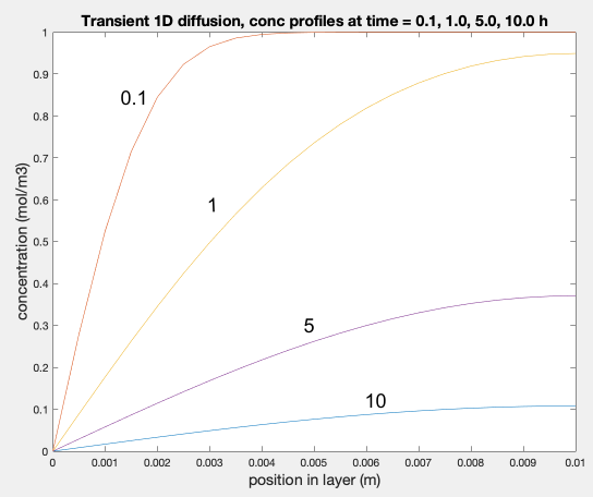
Diffusion This source code (link) solves a transient 1D diffusion problem, such as found in prescription drug patches. Students can vary parameters to see how closely the numerical approximation can approach the analytical solution of this problem. Other suggestions include computing the rate of diffusion out of the layer vs. time, and computing the fraction of the diffusing component left in the layer vs. time.
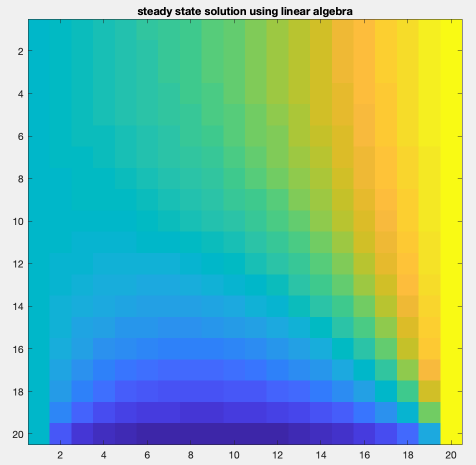
Heat Transfer This source code (link) solves a heat transfer system in several ways. The system is a 2D square body whose left side is at T=TL, right side is at T=TR, top side is insulated, and bottom side is exposed to heat transfer to a reservoir at T=TB. Students can change heat transfer parameters and the number of nodes, and can compute heat fluxes at the boundaries.
The steady state problem is solved by two methods: direct linear algebra solution (matrixNxN.m), as shown in the image below, in which TR > TL > TB, and a relaxation method (relaxNxN.m).
The transient solution from an initial condition is solved by two finite difference methods: a time-explicit method (explicitNxN.m) and a time-implicit method (implicitNxN.m).